
Key Takeaways
- The Brinson model decomposes a portfolio's excess return into three modeled effects: allocation, selection, and interaction.
- The choice between the Brinson-Hood-Beebower (BHB) and Brinson-Fachler (BF) variants is not trivial; the primary difference is how the allocation effect is calculated, which can materially change the attribution narrative even when the same underlying portfolio and benchmark data are used.
- Extending single-period Brinson attribution across multiple periods requires a linking algorithm to handle compounding effects; the choice of method can shift how contributions appear over time.
- Benchmark selection is often one of the most consequential inputs. A benchmark that doesn't fit the portfolio's strategy can produce attribution results that reflect benchmark misfit rather than genuine portfolio decisions, regardless of how precise the calculation is.
- For investment committees and CIOs, Brinson attribution can support performance review and implementation analysis, but it is not a substitute for direct holdings-based monitoring of portfolio drift or firm oversight processes.
Brinson attribution is one of the most widely referenced frameworks in performance analysis, providing a structured way to understand the sources of a portfolio's excess return. Yet, for many advisors and investment committees, a gap exists between understanding the concept and confidently applying it in practice. The choices surrounding its application, which decomposition variant, which benchmark, and which linking method, can materially change the story the numbers tell.
This isn't an academic problem; it's a practitioner's challenge. An advisor or CIO reviewing an attribution report needs to understand not just what the numbers say, but what assumptions produced them. A common misunderstanding is that the Brinson model measures manager skill; it measures the modeled decomposition of excess return relative to a chosen benchmark, and any inference about skill is closely tied to whether the inputs were appropriate for the strategy being evaluated.
This guide walks through the Brinson model from its foundational components to the methodological decisions that determine whether its outputs are meaningful or misleading. After reading, you will understand the math behind the model and the practitioner-level considerations needed to evaluate whether the analysis is sound.
What the Brinson Model Is and Where It Came From
The Brinson model is a holdings-based performance attribution framework that decomposes a portfolio's excess return relative to a benchmark into distinct modeled effects. At its core, it seeks to answer a simple but powerful question: did a portfolio outperform or underperform its benchmark because of its asset allocation decisions or its security selection decisions?
The framework's origins trace back to two seminal papers published in the Financial Analysts Journal . One, by Brinson and Fachler in 1985, and another, by Gary P. Brinson, L. Randolph Hood, and Gilbert L. Beebower in 1986, present closely related approaches to arithmetic performance attribution. Both remain foundational references in the development of brinson attribution. Originally designed for institutional equity portfolios segmented by asset class or sector, the model's enduring relevance comes from its intuitive logic.
It is important to distinguish Brinson attribution from other approaches like factor-based attribution. Brinson attribution decomposes returns by portfolio structure that is, by active weights and sector-level performance. In contrast, factor-based models decompose returns by a portfolio's exposure to systematic risk factors like value, growth, momentum, or size. The two frameworks are complementary; Brinson attribution explains where in the portfolio structure returns came from, while factor models can help explain why those returns occurred based on broader market dynamics.
While the model's core logic is straightforward, its apparent simplicity conceals meaningful methodological choices that the rest of this article will examine.
The Three Modeled Attribution Effects
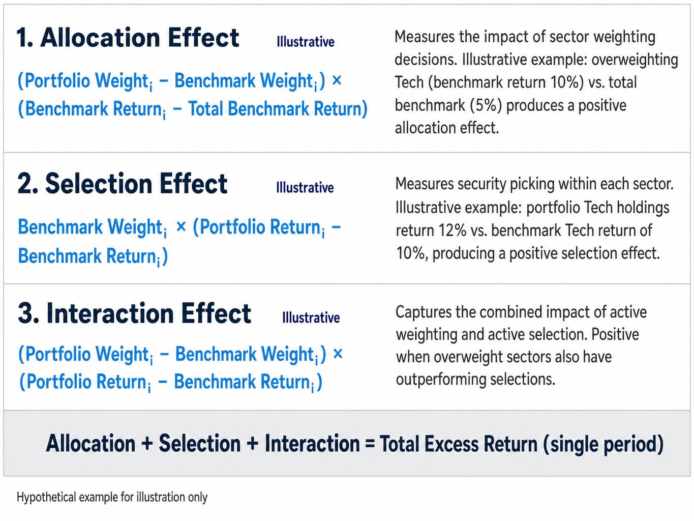
The Brinson model decomposes a portfolio's excess return into three primary modeled attribution effects: allocation, selection, and interaction. It is important to note that these are modeled effects that quantify structural differences between a portfolio and its benchmark; they do not necessarily reflect a portfolio manager's explicit intent.
To illustrate, consider a hypothetical two-sector portfolio (Tech and Healthcare) benchmarked against an index with the same sectors. We will use this simple example to walk through each effect. Because brinson attribution has multiple arithmetic formulations, it is also important to specify which version of the formulas is being used.
Allocation Effect
The allocation effect measures the return impact of a portfolio's sector or asset-class weighting decisions relative to the benchmark. Its exact formula depends on the attribution variant being used.
For a single sector, a common arithmetic Brinson-Fachler (BF)
specification is:
Allocation Effect (i) = (Portfolio Weight (i) - Benchmark Weight (i)) * (Benchmark Return (i) - Total Benchmark Return)
For a single sector, a common arithmetic Brinson-Hood-Beebower (BHB)
specification is:
Allocation Effect (i) = (Portfolio Weight (i) - Benchmark Weight (i)) * Benchmark Return (i)
For illustrative purposes, imagine the total benchmark returned 5%. The benchmark's Tech sector returned 10%, and the portfolio was overweight Tech compared to the benchmark. Under the BF formula, this overweight to a sector that outperformed the overall benchmark would generate a positive allocation effect. Under the BHB formula, the same active weight would be multiplied by the sector benchmark return directly. Both are valid arithmetic formulations, but they answer slightly different questions and therefore can produce different attribution narratives.
Selection Effect
The selection effect measures the return impact of security selection within each sector. It isolates whether the portfolio's holdings in a given sector performed better or worse than the benchmark's holdings in that same sector.
For a single sector, a common arithmetic formula is:
Selection Effect (i) = Benchmark Weight (i) * (Portfolio Return (i) - Benchmark Return (i))
Continuing the hypothetical example, if the portfolio's chosen tech stocks collectively returned 12% while the benchmark's tech sector returned only 10%, the portfolio would generate a positive selection effect. This quantifies the value added by picking specific securities that outperformed their sector peers.
Interaction Effect
The interaction effect is a cross-product term that captures the combined impact of active weighting and active selection decisions. It is positive when a portfolio overweights a sector in which it also picks outperforming securities, and negative when it overweights a sector where its selections underperform.
The formula for a single sector is:
Interaction Effect (i) = (Portfolio Weight (i) - Benchmark Weight (i)) * (Portfolio Return (i) - Benchmark Return (i))
This term is often the most difficult to interpret because it represents a joint effect. It is not noise, but its treatment and presentation differ across Brinson formulations.
In a single-period arithmetic analysis, these effects reconcile to total excess return when the decomposition is specified consistently and the underlying sector weights, sector returns, benchmark return, and classification mapping are internally aligned. When portfolio and benchmark segment weights each sum to 100%, the differences between BHB and BF allocation contributions offset in aggregate, although individual sector-level results can differ.
BHB vs. Brinson-Fachler: Why the Decomposition Choice Shapes the Attribution Narrative
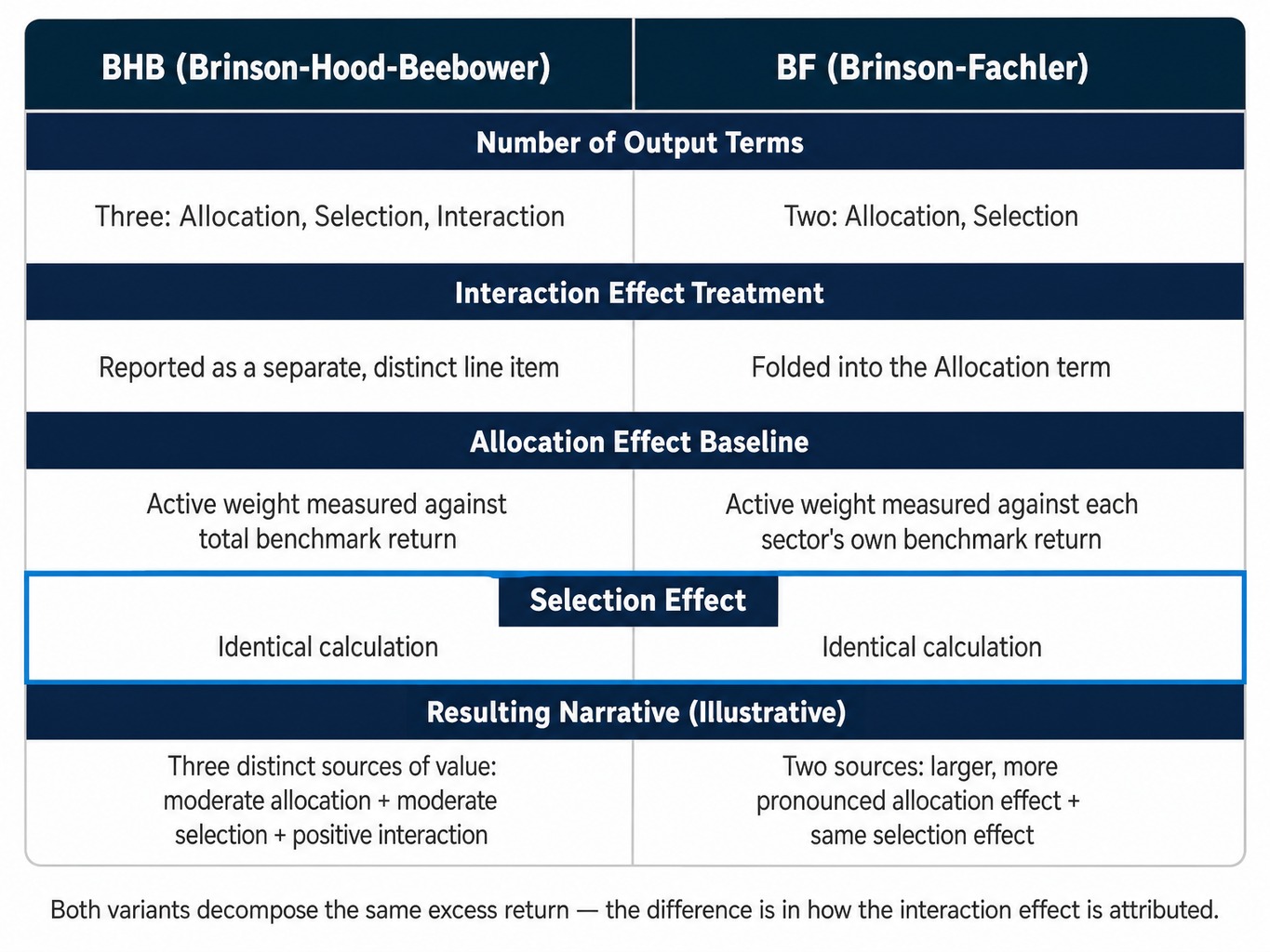
The Brinson-Hood-Beebower (BHB) and Brinson-Fachler (BF) models use the same underlying portfolio and benchmark data, but they define the allocation effect differently. This distinction can materially change the performance story an advisor or CIO reads from the same set of returns.
The primary structural difference is this:
- Brinson-Hood-Beebower (BHB): In a standard arithmetic specification, the allocation term uses the sector benchmark return directly.
- Brinson-Fachler (BF): In a standard arithmetic specification, the allocation term uses the sector benchmark return relative to the total benchmark return.
Stated as formulas for a single sector:
-
BHB allocation:
(Portfolio Weight (i) - Benchmark Weight (i)) * Benchmark Return (i) -
BF allocation:
(Portfolio Weight (i) - Benchmark Weight (i)) * (Benchmark Return (i) - Total Benchmark Return)
Both BHB and BF are commonly presented with allocation, selection, and interaction effects in arithmetic brinson attribution. The important point is not that one necessarily has interaction and the other does not, but that the allocation effect is defined differently, which changes how the results are interpreted.
Consider a hypothetical portfolio that overweights the Tech sector, where the sector benchmark return is above the total benchmark return and the portfolio's security selection also outperforms the Tech benchmark.
- Under the BHB model, the allocation effect is tied directly to the sector benchmark return, while selection and interaction capture the within-sector outperformance and the cross-product term.
- Under the BF model, the allocation effect is measured relative to how that sector performed versus the total benchmark, while selection and interaction continue to reflect within-sector outperformance and the joint effect.
The practical implication for advisors and CIOs is significant. When reviewing an attribution report, understanding which decomposition was used is necessary context. A report from one system showing a stronger or weaker allocation effect may be telling the same underlying return story through a different arithmetic lens. The underlying portfolio and benchmark data may be identical, but the narrative framing can differ because the allocation term is defined differently.
Extending Brinson Attribution Across Multiple Periods
Brinson attribution is mathematically defined for a single, discrete period. However, advisory firms and investment teams need to analyze performance over quarters, years, and custom reporting windows. This introduces a complexity that is often overlooked: simply summing single-period attribution effects rarely works.
The core problem is that returns compound geometrically, or multiplicatively, over time, while the standard Brinson decomposition is arithmetic, or additive, within each period. When you sum arithmetic effects across multiple periods, the result will almost never equal the portfolio's actual cumulative excess return. The difference is the attribution residual. This residual is not a rounding error; it is a mathematical artifact of the framework that can become material over longer horizons or in volatile markets.
To address this, the industry has developed several linking algorithms to distribute this residual across periods and effects, creating a smoother and more reconciled multi-period attribution. Commonly referenced approaches include:
- Carino Smoothing: A method that uses period-specific scaling factors together with an overall adjustment so the linked effects reconcile more closely to compounded multi-period results.
- Menchero Linking: A more complex method that distributes the residual based on the magnitude of each period's effects.
- Frongello Linking: Another approach that aims to provide a more intuitive allocation of the cross-period compounding effects.
An alternative is geometric attribution, which works with geometric excess returns from the start. Under an appropriately defined geometric framework, this can avoid the arithmetic compounding residual, but it still depends on consistent methodology and can produce effects that are less intuitive to interpret than arithmetic effects.
The practitioner takeaway is this: the linking method is not a footnote. It is a methodological choice that can shift how allocation and selection contributions appear over time. When reviewing multi-period attribution, knowing which linking approach was applied, and whether it is used consistently, is a crucial piece of analytical context.
Benchmark Selection: The Input That Shapes Every Attribution Output
Every Brinson attribution output is conditional on the benchmark chosen, yet benchmark selection often receives less scrutiny than the attribution results themselves. An attribution analysis is only as good as its benchmark, and a structural mismatch between the portfolio and its benchmark can produce results that are mathematically correct but analytically misleading.
This is a scenario many investment committees have faced. Consider a mid-size RIA where the investment committee ran Brinson attribution on the same balanced portfolio against two different benchmarks: a blended 60/40 policy benchmark and a single multi-asset index. The allocation effect for the equity sleeve flipped from positive to negative depending solely on which benchmark was selected. The attribution outputs were never wrong; the input assumption had simply shifted.
A growth-tilted equity portfolio benchmarked against a broad market index, for example, will likely show a persistent positive allocation effect toward growth sectors. This may reflect a structural benchmark mismatch rather than a series of successful active allocation decisions. Similarly, for multi-asset portfolios, differences in how sectors or geographic regions are classified between the portfolio accounting system and the benchmark provider can shift attribution results without any change in the underlying holdings.
The key takeaway for practitioners is foundational: before interpreting any Brinson attribution report, the first step is to evaluate the benchmark. Does it appropriately reflect the portfolio's investment mandate, style, and constraints? If not, the attribution analysis risks becoming an exercise in measuring benchmark misfit rather than a genuine decomposition of excess return.
Applying Brinson Attribution Beyond Equities
The Brinson model was originally designed for equity portfolios segmented by sector, but practitioners have adapted it for fixed-income and multi-asset contexts. However, these adaptations come with limitations.
For fixed-income portfolios, the framework is often adapted by decomposing returns by duration bucket, credit quality (e.g., investment grade vs. high yield), or issuer sector. While this can provide some insight, the standard Brinson model does not natively capture the primary drivers of fixed-income returns, such as yield-curve positioning, spread changes, and convexity effects. More specialized fixed-income attribution models, which decompose returns into carry, curve, and spread components, may provide more granular and meaningful analysis for bond-heavy portfolios.
For alternative investments, the limitations are more pronounced. Illiquid holdings, infrequent valuations, and the absence of a meaningful, investable benchmark make a standard Brinson decomposition difficult to apply. These limitations can make attribution results less reliable or more difficult to interpret.
Brinson attribution remains a powerful and useful framework for the equity and traditional multi-asset portions of a client's portfolio. However, firms managing portfolios with significant fixed-income or alternative allocations may want to evaluate whether supplementary attribution approaches provide a more complete picture of performance drivers.
Using Brinson Attribution as a Governance and Consistency Tool
Beyond explaining historical performance, Brinson attribution can support governance and consistency reviews for multi-advisor firms. For Chief Investment Officers (CIOs) and investment committees, attribution analysis may help highlight performance differences associated with active weights and security selection across accounts that are expected to track a common model or philosophy.
For illustrative purposes, imagine an investment committee establishes a model portfolio with specific target sector allocations. Running Brinson attribution across multiple advisor-managed accounts against that model as the benchmark may surface recurring patterns in benchmark-relative results. For example, the analysis may show that one advisor's accounts repeatedly display positive or negative allocation effects in a particular sector, while another advisor's accounts show repeated selection differences tied to substitute holdings. These patterns can be useful for review, but they are not a substitute for direct holdings-based drift monitoring, transaction review, or the firm's own oversight processes.
This use case shifts attribution from a backward-looking performance explanation to a consistency-oriented analytical lens. It can help investment leadership evaluate whether benchmark-relative results line up with the firm's intended implementation across teams and offices. When attribution results vary because different benchmarks, decomposition variants, or reporting conventions are used, firms may end up with inconsistent analytical narratives across advisors. That is the broader workflow challenge relevant here, establishing a shared analytical and presentation baseline across portfolio comparisons and reporting processes.
The practical challenge, of course, is producing consistent analysis at scale, comparing large numbers of portfolios, working from complete portfolio data, and presenting the results in a format that supports oversight.
Read more: Standardize Advisory Workflows for Enterprise Growth | VRGL
How VRGL Supports Consistent Portfolio Analysis and Comparisons
Brinson attribution and comparative portfolio analysis are related but distinct. Specialized attribution systems are used to calculate benchmark-relative performance effects such as allocation, selection, and interaction. VRGL is positioned differently. It supports consistent portfolio analysis, comparisons, and presentation workflows that can complement a firm's broader analytical process.
The VRGL Growth Platform is designed to support this kind of operational infrastructure. Discovery and fact-finding remain with the advisor. Once portfolio information has been gathered, VRGL's workflow begins with AI-powered extraction from supported investment statements.
From there, advisors and investment teams can compare current portfolios against proposed portfolios across five pillars: performance, risk, diversification, taxes, and fees.
For firms focused on producing consistent portfolio comparisons and client-ready materials, VRGL's workflow moves from data intake to structured comparison to branded, governed presentation materials. This helps reduce the manual preparation that typically sits between raw portfolio data and a client-ready or committee-ready report . For enterprise firms, VRGL's configurable governance layer supports consistency across advisors and teams without dictating how individual advisors interpret or present results.
VRGL does not replace an advisor's analytical judgment or fiduciary responsibility. Instead, it provides the data, analytics, and workflow infrastructure that can support more consistent and efficient preparation, allowing advisors to focus on interpreting the results and communicating their value.
See how VRGL's Comparative Portfolio Analysis supports your acquisition workflow
Conclusion
Brinson attribution is not just a formula: it is a chain of methodological decisions. The value of any attribution output depends on the quality of those decisions. While the model decomposes excess return into allocation, selection, and interaction effects, the chosen decomposition variant, benchmark, linking method, and classification methodology all shape the story the numbers tell.
For advisory firms, the challenge extends beyond understanding the math to ensuring analytical methods are consistently applied, results are appropriately interpreted, and portfolio insights are communicated clearly to clients and investment committees. Firms that treat attribution as a governed analytical workflow, rather than an ad-hoc calculation, are better positioned to use it as both a client communication tool and an internal consistency check.
This article is for informational purposes only and should not be considered investment, legal, or compliance advice. The information contained herein is not a substitute for professional advice, and all investment decisions should be made in consultation with a qualified financial advisor.
Frequently Asked Questions
Why does Brinson attribution sometimes produce a residual that does not reconcile to total excess return?
A residual typically appears in multi-period attribution when single-period arithmetic effects are summed without a linking algorithm. Because returns compound geometrically while arithmetic attribution effects do not, the sum diverges from the actual multi-period excess return. Applying a linking method like Carino or Menchero smoothing can distribute this residual and restore reconciliation.
How does geometric attribution differ from arithmetic attribution in the Brinson framework?
Arithmetic attribution calculates each effect as an additive contribution to excess return, which is intuitive but creates compounding residuals over multiple periods. Geometric attribution works with geometric excess returns, which compound more naturally across periods. The trade-off is that geometric attribution effects are often less intuitive to interpret and still depend on a consistent methodology.
What is the relationship between Brinson attribution and GIPS presentation standards?
The Global Investment Performance Standards (GIPS), administered by CFA Institute, do not mandate a specific attribution methodology. However, firms presenting attribution in GIPS-compliant composites may want to disclose the methodology used, including the decomposition variant and linking approach, to support the transparency objectives that GIPS standards emphasize.
Can different holdings-based inputs produce different Brinson attribution results for the same portfolio?
Yes. Brinson attribution is generally a holdings-based framework, and results can differ when the underlying inputs differ. Changes in holdings snapshot dates, valuation timing, treatment of cash flows, transaction timing, or security-to-sector classification can all affect weights, segment returns, and the resulting attribution effects, even for the same account over the same general period.
How does Brinson attribution complement factor-based attribution rather than replace it?
Brinson attribution decomposes returns by portfolio structure, sector weights, and security selection. Factor-based attribution decomposes returns by exposure to systematic risk factors like value or momentum. Brinson explains where returns came from structurally, while factor models help explain why returns behaved as they did relative to common risk exposures.
What challenges arise when applying Brinson attribution to portfolios with unclassified or illiquid holdings?
Holdings that do not map cleanly to benchmark sectors, such as private investments or structured products, create classification gaps that can distort attribution results. These holdings may be assigned to a residual category or force-fitted into an imprecise sector, either of which introduces attribution noise and may require supplementary analysis.